2. Introducing Discrete Mathematics
2.1. Course Objectives
At Georgia Gwinnett College, students who have successfully completed the Discrete Mathematics course will,
-
Reason mathematically and use mathematical language appropriately to demonstrate an understanding of comprehending and constructing mathematical arguments.
-
Perform combinatorial analysis to solve counting problems and analyze algorithms.
-
Demonstrate an understanding of discrete structures including sets, permutations, relations, graphs, and trees.
-
Demonstrate algorithmic thinking using mathematical creativity and critical thinking by specifying algorithms, verifying that algorithms work, and analyzing the time required to perform specific algorithms.
-
Use appropriate technology in the evaluation, analysis, and synthesis of information in problem-solving situations.
These course goals help structure the content of this class, which is aimed at students of information technology, computer science, and applied mathematics. The focus is on applying discrete math techniques from the two broad component areas of discrete math, namely combinatorics or enumerative techniques, and graph theory.
To that end, algorithmic thinking figures prominently in this course. Designing algorithms, particularly algorithms applied to networks, involves the use of graph theory methods. Implementing algorithms requires a careful understanding of logical structures, and usually a top down implementation approach, beginning with a specifications description, and then proceeding to a pseudocode implementation and finally a language dependent coding implementation. Moreover, analyzing the complexity of algorithms requires a knowledge of functions, the growth of functions, and counting techniques from combinatorial analysis. Similarly, mathematical induction and recursive definitions are used in a cohesive way to understand algorithms and the options in implementing these recursively versus iteratively.
The approach we take is one with an integrative incorporation of programming and algorithms into the course. The aim is to help improve students success with their broad programming curricula in courses like Intermediate and Advanced Programming.
2.2. Applications of Discrete Mathematics
Discrete mathematics is applied in many areas including the physical, engineering, and increasingly, the social sciences.
2.2.1. Applications to Applied Mathematics
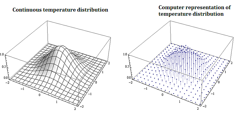
Most problems that involve computational methods, need to be solved using computers. Rather than solve for the temperature map of an entire planar region, we solve for the temperature using a discrete set of mesh or grid of points on a representative subset of the planar region.
2.2.2. Applications to Information Technology and Computer Science
Discrete mathematics is needed for computer science as information and data is stored digitally. Digitally represented data is inherently discrete and is processed using discrete methods. For example a course grid discrete representation of the 2-d temperature distribution from the plate above could be:
\( \left(\begin{matrix}1&1&1\\2&4&8\\3&9&27\\4&16&64\\5&25&125\\\end{matrix}\right) \)
A voter registry may have voters in a database accessible from a list:
\( \left(\begin{matrix}John\ Smith\\Raheem\ Johnson\\.\\.\\.\\Sarah\ Muller\\\end{matrix}\right) \)
Which may need to be accessed and sorted, say geographically or alphabetically.
2.2.3. Applications to Data Science
Data science solutions to many problems use machine learning algorithms that are inherently discrete in nature. The information that needs processing is discrete, as are the basic problems in data science such as classification or clustering problems. In particular
-
Information consisting of data sets is represented using various data structures including graphical structures such as trees. Data science methods and algorithms involve procedures that manipulate these graphical structures to, for example, networks, classification trees, and decision trees.
-
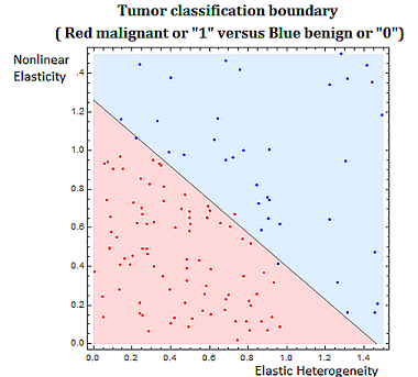
Classification problems are discrete in nature. Classifying tumors as malignant or as benign involves trying to predict if a variable \(Y\) that we can think of as taking on two values either \(0\) or \(1\) either malignant or benign. There are various algorithms used in classification problems, such as the binary tumor classification, including methods from probability.
2.2.4. Applications to Engineering
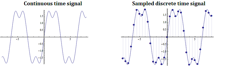
Digital signal processing involves taking a video, audio, or other signal like temperature, pressure, position and velocity, which is continuous, digitizing it and then processing the digital signal mathematically.
2.2.5. Applications of Combinatorics
Combinatorics involves in part the study of counting the number of objects, satisfying a specified condition, from sets of variable size. Enumeration and combinatorics is important in many areas and examples including:
-
Calculating the number of steps an algorithm needs to process a data set of variable size \(𝑛\). This problem is called the computational cost of the algorithm as a function of \(𝑛\).
-
Calculating the possible number of codes in a cryptographic code system
2.2.6. Applications of Graph Theory
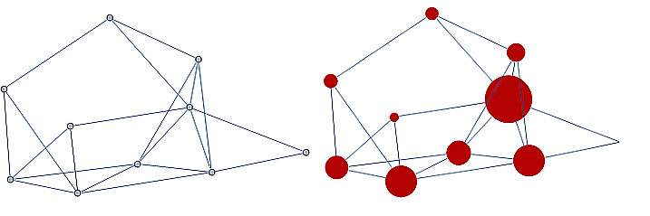
Graph theory , which is the study of structures constructed with nodes and the edges joining them, has applications in many fields including,
-
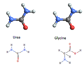
Chemistry - representing molecular bonding and structure
-
Information technology and computer science - ranking pages on the internet, with pages considered as nodes and page links as edges.
-
Industrial engineering and network optimization
-
Traffic routes (computer, internet, air, highway, subway systems) can be represented with stations as nodes and connections as edges.
-
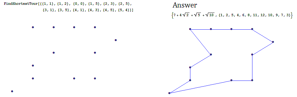
Often we are interested in finding an optimal path in a network such as in the following example, finding the shortest tour over a series of towns on a map.
-
An example of the shortest tour problem, is shown below, using a software solution.
2.2.7. Applications of Probability and Statistics
Many probability assignments are based on counting and combinatorial methods.
-
If we assume that the likelihood of rain is the same on any day in the month of September, we might be interested in the probability that it rains on \(0\) days, it rains on exactly \(1\) day, exactly \(2\) days, etc. Such probability assignments are called discrete distributions, by contrast with continuous distributions like the bell curve.
-
Also probability and statistical techniques are often used in data science. The binary classification problem, of say classifying a tumor as malignant or benign, uses a statistical modeling technique, called regression, specifically logistic regression to determine the strength of the relationship between the independent variable, and dependent heterogeneity variable. In the tumor grading example the independent variable would be \((x_1,x_2 )\) (elastic heterogeneity, nonlinear elasticity), and the dependent variable would be \(Y\), classified as \(0\), or \(1\), (malignant or benign).
2.2.8. Applications to Social Sciences
Discrete mathematical techniques are important in understanding and analyzing social networks including social media networks.
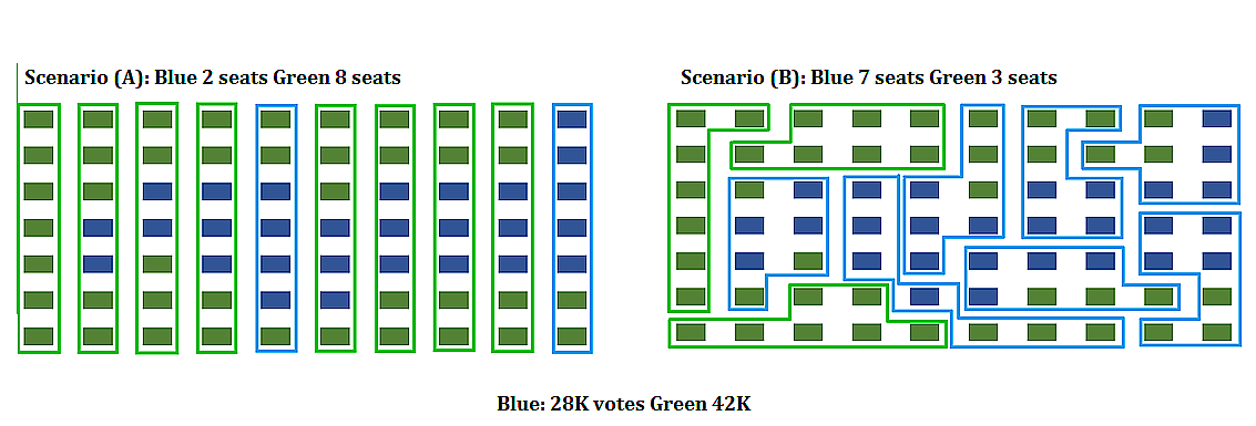
The mathematics of voting is a thriving area of study, including mathematically analyzing the gerrymandering of congressional districts to favor and/or disfavor competing political parties. The following example illustrates some of the fundamental ideas related to gerrymandering.
Consider a fictitious state made up of \(10\) congressional districts with \(7\) thousand voters in each district. To win a district a party (Green or Blue) needs to win \(4\) thousand or more votes. Consider the following two districting map scenarios. In each scenario, the blue party earns \(28\) thousand votes, and the green party earns \(42\) thousand votes. In scenario \(A\), the blue party wins \(2\) out of \(10\) districts, but in scenario \(B\) it wins \(7\) out of \(10\) districts.
2.3. Understanding Continuous and Discrete Sets
Sets of objects are discrete if there is a gap between each of the elements. Informally we mean that the elements are not connected continuously so that there the values of the set elements do not fall on a continuum. Practically speaking, sets are discrete if they can be counted.
|
A finite set is always discrete, since it can be counted. |
2.3.1. Examples of discrete sets
There are various types of discrete sets.
The set of all real numbers is a continuous set, and cannot be counted (said to be uncountable).
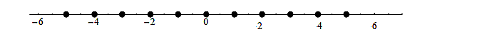
By contrast the set of integers, both negative and positive, \(..., -6, -5, -4, -3, -2, -1, 0, 1, 2, 3, 4, 5, 6,...\), is countable and discrete.
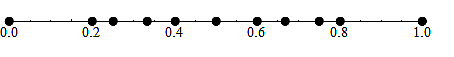
The set of all fractions or rational numbers in the interval \([0,1\)] is countable, by contrast, with the set of all real numbers in the continuous interval, \([0,1\)], which is uncountable and also not discrete.
2.4. Exercises
-
Give the set of all relations from the set \(\{A, B \}\) to the set, \(\{0, 1, 2\}\), and explain why the set is discrete.
-
Consider rolling a six-sided die twice. The possible outcomes are of the form \((2, 3)\), corresponding to rolling a \(2\), followed by rolling a \(3\), or \((3,2)\), corresponding to rolling a \(3\), followed by a \(2\).
-
List all possible outcomes.
-
Explain why the set of all possible outcomes is a discrete set.
-