Discrete Math

12.1. Introduction and Basic Definitions

A graph \(G=\left(V,\ E\right)\) is a structure consisting of a set of objects called vertices \(V\) and a set of objects called edges \(E\). An edge \(e\in\ E\) is denoted in the form \(e=\left\{x,y\right\}\), where the vertices \(x,y\in\ V\). Two vertices \(x\) and \(y\) connected by the edge \(e=\left\{x,y\right\}\), are said to be adjacent , with \(x\) and \(y\),called the endpoints.

A simple graph is one in which there are no loops (edges joining the same vertex) and no two edges joining the same pair of vertices. The graphs we consider are assumed to be simple unless stated otherwise.

Example 1 - an undirected graph.

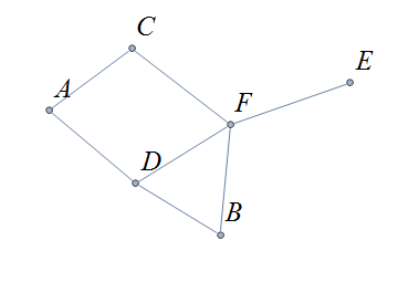
The graph shown has vertex set \(V=\left\{A,\ B,\ C,\ D,\ E,\ F\right\}\) and edge set \(E=\{\{A,C\},\{A,D\},\{B,D\}\{B,F\},\{C,F\},\{D,F\},\{F,E\}\}\)

A directed graph (or digraph ) is an extension of the definition of a graph in which the edges are recognized to be ordered.

Example 2 - a directed graph.

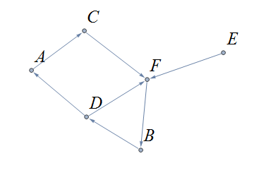
The graph \(G=(V,E)\) with vertex set \(V=\{A,B,C,D,E,F\}\) and edge set \(E=\{\{A,C\},\{D,A\},\{B,D\}\{F,B\},\{C,F\},\{D,F\},\{F,E\}\}\) with edge set considered as ordered is a directed graph and shown below.

The degree of a vertex \(v \in V\), denoted \(d(v)\), is the number of edges in the graph \(G\) containing the vertex \(v\).

Example 3

The degrees of each of the vertices in the undirected graph \(G\) with vertex set \(V=\{A,B,C,D,E,F,G\}\) and edge set \(E=\{\{A,C\},\{A,D\},\{B,D\}\{B,F\},\{C,F\},\{D,F\},\{F,G\}\) are,

\(d\left(A\right)=2\)

\(d\left(B\right)=2\)

\(d\left(C\right)=2\)

\(d\left(D\right)=3\)

\(d\left(E\right)=0\)

\(d\left(F\right)=4\)

\(d\left(G\right)=1\)

Notice that the total sum of all the degrees \(d\left(A\right)+\ d\left(B\right)\ +\ d\left(C\right)+\ \ d\left(D\right)\ \ +d\left(E\right)+\ d\left(F\right) + d\left(G\right)=14\) is twice the number of edges \(\left|E\right|=7\) in the graph. This is true in general and we state this result as theorem, often called the handshaking lemma.

Handshaking Lemma

The sum of the degrees of the vertices of a graph \(G=\left(V,\ E\right)\) is equal to twice the number of edges in \(G\). That is, \(\displaystyle \sum_{v\in V}{d\left(v\right)=2\ \left|E\right|}\).

A useful consequence of this to keep in mind is that the sum of the degrees of a graph is always even.

12.2. Representing graphs.

In addition to the vertex-edge representation of graphs there are alternative ways to represent a graph, especially useful for computing.

12.2.1. The Adjacency Matrix

One way is the use of an adjacency matrix. The adjacency matrix \(M\) represents a graph in a table form, containing a row and column for each vertex \(v_i\). If the vertices \(v_i\) and \(v_j\) are connected by an edge \(e\), the adjacency matrix will contain a \(1\) in the \(i-th\) row and \(j-th\) column and \(0\) otherwise. Denoting by \(m_{i,\ j}\) the component of the adjacency matrix in the \(i-th\) row and \(j-th\) column, we define the adjacency matrix for the graph \(G=\left(V,E\right)\) as

\( m_{i,j}=\left\{ \begin{array}{cc} 1 & \text{if}\text{ }\left\{v_i,v_j\right\} \text{is}\text{ }\text{in}\text{ }E\text{ } \\ 0 & \text{otherwise} \end{array} \right. \)

Example 4 - adjacency matrix of a graph

The graph with vertex set \(V=\left\{A,\ B,\ C,\ D,\ E,\ F\right\}\) and edge set \(E=\{\{A,C\},\{A,D\},\{B,D\}\{B,F\},\{C,F\},\{D,F\},\{F,E\}\}\) has adjacency matrix

\begin{matrix}A&0&1&1&0&0&0\\C&1&0&0&0&1&0\\D&1&0&0&1&1&0\\B&0&0&1&0&1&0\\F&0&1&1&1&0&1\\E&0&0&0&0&1&0\\\ &A&C&D&B&F&E\\\end{matrix}

Example 5 - obtaining the graph from the adjacency matrix

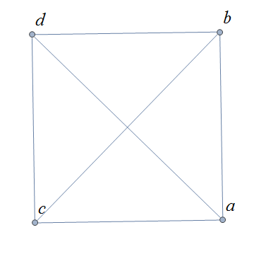
The graph with adjacency matrix

\begin{matrix}a&0&1&1&1\\c&1&0&1&1\\d&1&1&0&1\\b&1&1&1&0\\\ &a&c&d&b\\\end{matrix}

is the graph shown below.

12.2.2. The Adjacency Matrix for Directed Graphs

Undirected graphs are represented using symmetric adjacency matrices while digraphs are represented by adjacency matrices that are not symmetric.

Example 6 - adjacency matrices for an undirected graph and for a directed graph

In the figure below the first graph is undirected while the second is a digraph.

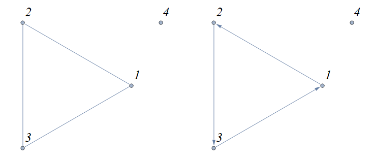
Their adjacency matrices are respectively,

\( \left(\begin{matrix}0&1&1&0\\1&0&1&0\\1&1&0&0\\0&0&0&0\\\end{matrix}\right) \) and \( \left(\begin{matrix}0&1&0&0\\0&0&1&0\\1&0&0&0\\0&0&0&0\\\end{matrix}\right). \)

12.3. Weighted Graphs

A weighted graph is one in which each edge \(e\) is assigned a nonnegative number \(w(e)\), called the weight of that edge. Weights are typically associated with costs, or capacities of some type like distance or speed. The adjacency matrices for weighted graphs are very similar to those for graphs that are not necessarily weighted. Instead of using a \(1\) to represent an edge between two vertices, say \(v_i\), and \(v_j\), we place the the weight of the edge \(w(e)\) in position \(m_{i,j}\) of the adjacency matrix as shown in the following two examples.

Example 7

Consider first the following weighted undirected graph

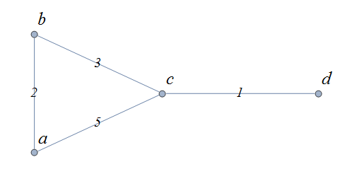
Its adjacency matrix is \( \left(\begin{matrix}0&2&5&0\\2&0&3&0\\5&3&0&1\\0&0&1&0\\\end{matrix}\right). \)

By contrast, the directed weighted graph below

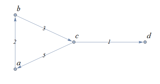
has adjacency matrix \( \left(\begin{matrix}0&2&0&0\\0&0&3&0\\5&0&0&1\\0&0&0&0\\\end{matrix}\right). \)

12.4. Subgraphs

A graph \(H=(V_1,E_1)\) is said to be a subgraph of the graph \(G=(V,\ E)\) if \(V_1\subseteq V\) and \(E_1\subseteq E\).

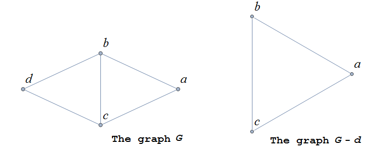
If the vertex \(v\in V\) belongs to the graph \(G=(V,E)\), we denote by \(G-v\) , the subgraph obtained from G by removing the vertex \(v\) and all edges in \(E\) adjacent to the vertex \(v\).

Below is shown a graph \(G\), and the subgraph \(G-d\) formed by removing the vertex \(d\).

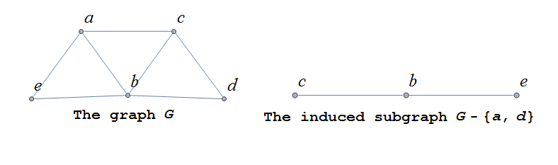
A natural generalization of the subgraph obtained by removing a vertex is the subgraph obtained by removing multiple vertices and the edges associated with the removed vertices. The subgraph obtained is called the subgraph induced by removing those vertices.

Example 8

Below is a graph \(G(V,E)\) and the subgraph obtained by \(V-\{a,d\}\), called the induced subgraph \(G-\{a,d\}\), with a slight abuse of notation

12.5. Connectivity, Eulerian Graphs, and Hamiltonian Graphs

A walk on a graph \(G=\left(V,E\right)\) is a finite, non-empty, alternating sequence of vertices and edges of the form, \(v_0e_1v_1e_2\ldots e_nv_n\), with vertices \(v_i\in V\) and edges \(e_i\in E\).

A trail is a walk that does not repeat an edge, ie. all edges are distinct.

A path is a trail that does not repeat a vertex.

The distance between two vertices, \(u\) and \(v\), denoted \(d(u,v)\), is the number of edges in a shortest path connecting them.

A cycle is a non-empty trail in which the only repeating vertices are the beginning and ending vertices, \(v_0=v_n\).

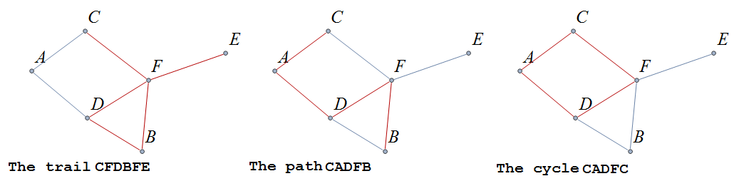
In the graphs below the first shows a trail \(CFDBFE\). It is not a path since the vertex \(F\) is repeated. The second shows a path \(CADFB\), and the third a cycle \(CADFC\). Also note the following distances, \(d(A,D)=1\), while \(d(A,F)=2\), and \(d(A,E)=3\).

A graph is connected if there is a path from each vertex to every other vertex.

The graph below is not connected,

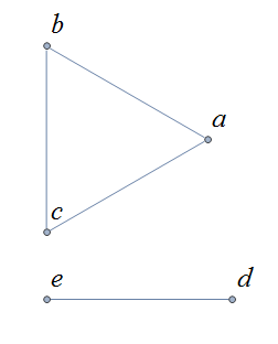
and has adjacency matrix,

\( \left(\begin{matrix}0&1&1&0&0\\1&0&1&0&0\\1&1&0&0&0\\0&0&0&0&1\\0&0&0&1&0\\\end{matrix}\right). \)

12.5.1. Eulerian Graphs

Informally an Eulerian graph is one in which there is a closed (beginning and ending with the same vertex) trail that includes all edges. To define this precisely, we use the idea of an Eulerian trail.

An Eulerian trail or Eulerian circuit is a closed trail containing each edge of the graph \(G=(V,\ G)\) exactly once and returning to the start vertex. A graph with an Eulerian trail is considered Eulerian or is said to be an Eulerian graph .

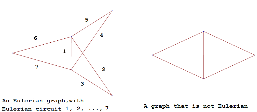
In the following, the first graph is Eulerian with the Eulerian circuit sequenced from \(1\) to \(7\). The second is not an Eulerian graph. Convince yourself of this fact by looking at all necessary trails or closed trails.

An Euler path on a graph is a path that uses each edge of the graph exactly once. The following are useful characterizations of graphs with Euler circuits and Euler paths and are due to Leonhard Euler

Theorem on Euler Circuits and Euler Paths

A finite connected graph has an Euler circuit if and only if each vertex has even degree.
A finite connected graph has an Euler path if and only if it has most two vertices with odd degree.

12.5.2. Hamiltonian Graphs

A cycle in a graph \(G=\left(V,E\right)\), is said to be a Hamiltonian cycle if every vertex, except for the starting and ending vertex in \(V\), is visited exactly once.

A graph is Hamiltonian , or said to be a Hamiltonian graph , if it contains a Hamiltonian cycle.

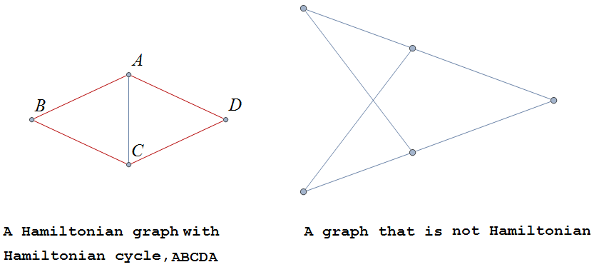
The following graph is Hamiltonian and shows a Hamiltonian cycle \(ABCDA\), highlighted, while the second graph is not Hamiltonian.

While we have the Euler Theorem to tell us which graphs are Eulerian or not, there are no comparable simple criteria to determine if graphs are Hamiltonian or not. We do have the following sufficient criterion due to Paul Dirac.

Theorem (Dirac) on Hamiltonian graphs

A simple graph, with \(n≥3\) vertices, is Hamiltonian if every vertex \(v\) has degree \(d(v)\geq \frac{n}{2}\).

12.6. Exercises

For each of the following graphs, find their
1. Adjacency matrices
2. Adjacency lists
For each of the following digraphs, find their
1. Adjacency matrices
2. Adjacency lists
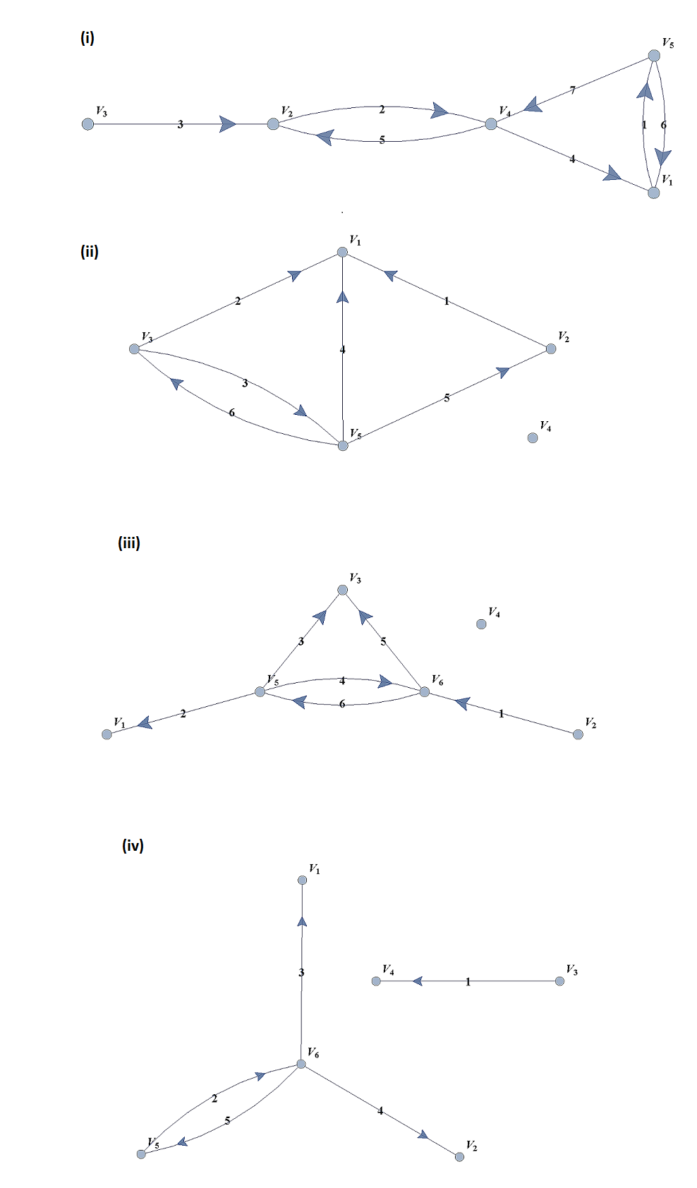
Draw, with labeled edges and vertices, the graphs given by the following adjacency matrices.
1. \( \) \( \left( \begin{matrix}0&1&0&1&1\\1&0&1&1&0\\0&1&0&0&0\\1&1&0&0&0\\1&0&0&0&0\\\end{matrix} \right) \)
2. \( \) \( \left( \begin{matrix}0&1&1&0&1\\1&0&0&0&0\\1&0&0&0&0\\0&0&0&0&1\\1&0&0&1&0\\\end{matrix} \right) \)
3. \( \) \( \left( \begin{matrix}0&0&0&1&0&0\\0&0&1&0&0&1\\0&1&0&0&1&1\\1&0&0&0&0&0\\0&0&1&0&0&0\\0&1&1&0&0&0\\\end{matrix} \right) \)
4. \( \) \( \left( \begin{matrix}0&1&0&0&1&1\\1&0&0&0&1&1\\0&0&0&0&0&0\\0&0&0&0&1&1\\1&1&0&1&0&0\\1&1&0&1&0&0\\\end{matrix} \right) \)
Draw, with labeled edges and vertices, the digraphs given by the following adjacency matrices
1. \( \) \( \left( \begin{matrix}0&1&1&0&0\\0&0&0&0&1\\0&1&0&0&0\\1&0&1&0&1\\0&1&0&0&0\\\end{matrix} \right) \)
2. \( \) \( \left( \begin{matrix}0&1&1&0&1\\1&0&0&0&0\\1&0&0&0&0\\0&0&0&0&1\\1&0&0&1&0\\\end{matrix} \right) \)
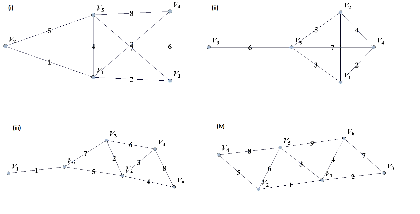
Draw, with labeled edges and vertices, the weighted graphs (or digraphs) given by the following adjacency matrices.
1. \( \) \( \left( \begin{matrix}0&10&3&0&5\\10&0&2&3&0\\3&2&0&7&4\\0&3&7&0&1\\5&0&4&1&0\\\end{matrix} \right) \)
2. \( \) \( \left( \begin{matrix}0&2&3&4\\0&0&5&7\\0&0&0&6\\5&8&8&0\\\end{matrix} \right) \)
3. \( \) \( \left( \begin{matrix}0&0&0&1&0&0\\0&0&1&0&0&1\\0&1&0&0&1&1\\1&0&0&0&0&0\\0&0&1&0&0&0\\0&1&1&0&0&0\\\end{matrix} \right) \)
4. \( \) \( \left( \begin{matrix}0&5&3&2&5\\0&0&0&0&0\\8&2&0&5&4\\0&1&0&0&1\\0&0&0&1&0\\\end{matrix} \right) \)
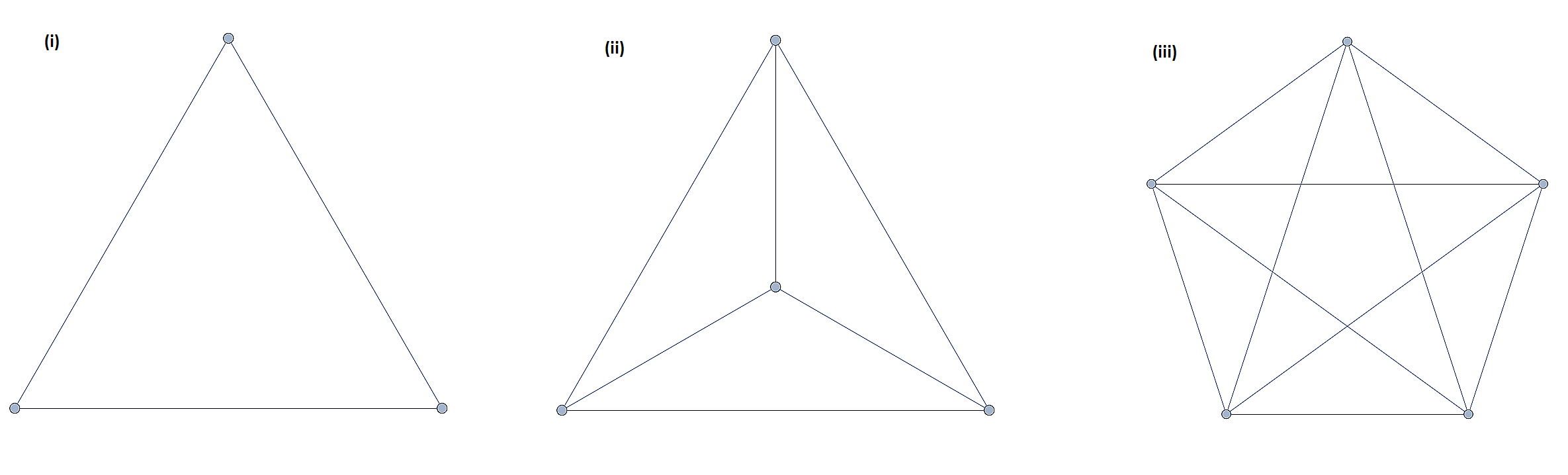
The complete graph \(K_n\) is the graph with \(n\) vertices and edges joining every pair of vertices. Draw the complete graphs \(K_2,\ K_3,\ K_4,\ K_5,\) and \(K_6\) and give their adjacency matrices.
The path graphs \(P_n\) are connected graphs with \(n\) vertices (vertex set \(V={v_1,v_2,\ldots,\ v_n}\)) and with \(n-1\) edges (edge set \(E=\{\{v_1,v_2\},\{v_2,v_3\},\{v_3,v_4\},...,\{v_{n-1},v_n\} \}\)). Draw the path graphs \(P_2,\ P_3,\ P_4,\ P_5,\) and \(P_6\) and give their adjacency matrices.
Regular graphs are graphs in which all the vertices have the same degree. A graph in which all vertices have degree \(k\) is called a \(k-\)regular graph.
1. Describe all \(0-\)regular, \(1-\)regular, and \(2-\)regular graphs.
2. Explain using the handshaking lemma why all \(3-\)regular graphs must have an even number of vertices.
3. Explain why all the complete graphs \(K_n\) are regular.
4. Draw a \(3-\)regular graph with 8 vertices and give its adjacency matrix.
A graph \(G=G(V,E)\) is said to be bipartite if its vertex set, \(V\), can be partitioned into two disjoint sets \(M\) and \(N\), with \(V=M\cup N\), so that every edge \(e\in E\) joins two vertices, with one vertex in \(M\) and the other in \(N\). One way to think of bipartite graphs is to partition the vertices by two colors, say black and white, and every edge connects a black vertex with a white vertex (never connecting two vertices of the same color).
1. Show that the following are bipartite graphs by explicitly partitioning them using a coloring scheme to partition the vertices.
2. Explain why the following are not bipartite graphs.
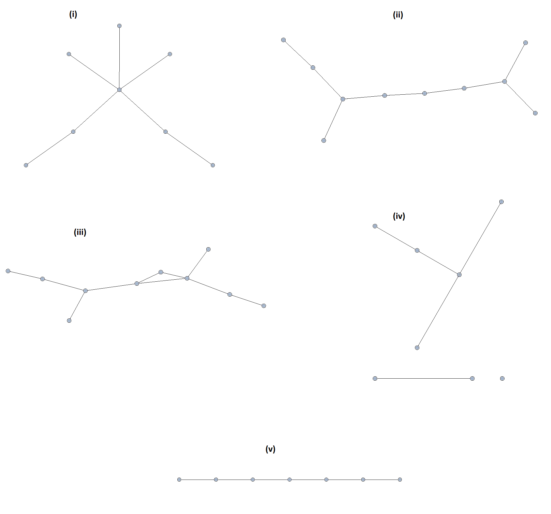
A tree is a connected graph with no cycles. It can be shown, using mathematical induction, that a tree with \(n\) vertices must have exactly \(n-1\) edges. Determine which of following graphs are trees and which are not. Explain your reasoning.
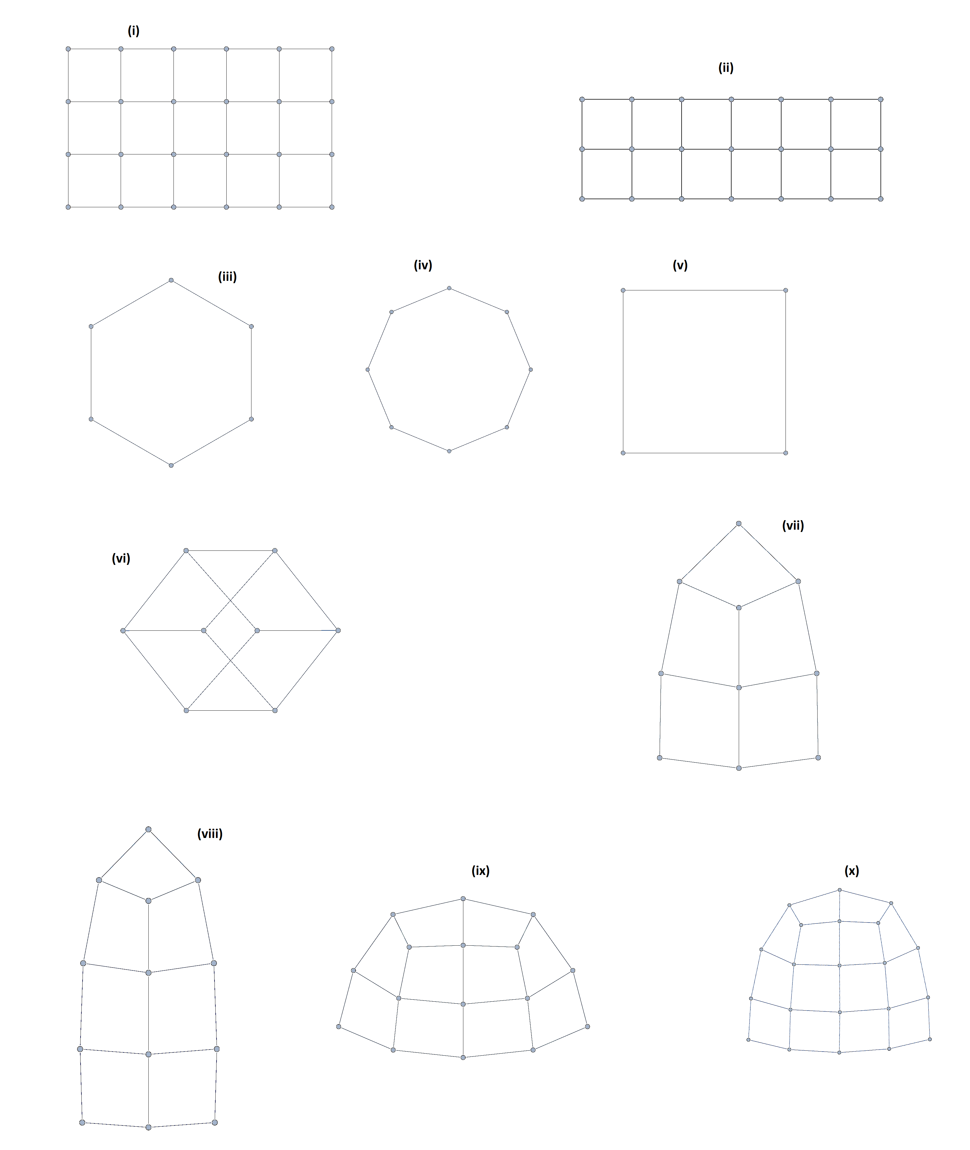
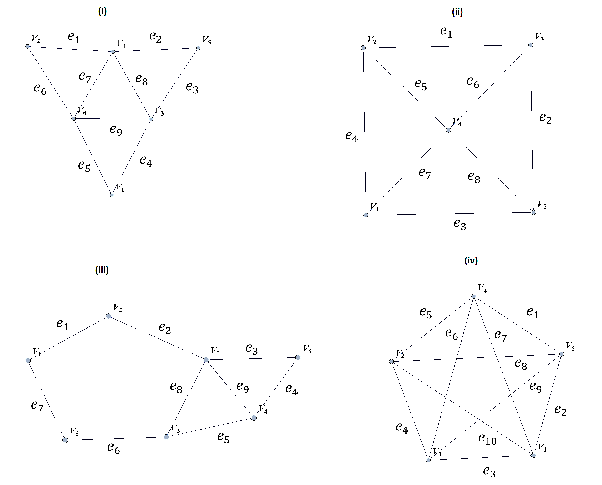
Use the Euler Theorem to determine which of the following graphs are Eulerian (have Euler circuits). For those graphs that are Eulerian, give an Eulerian circuit.
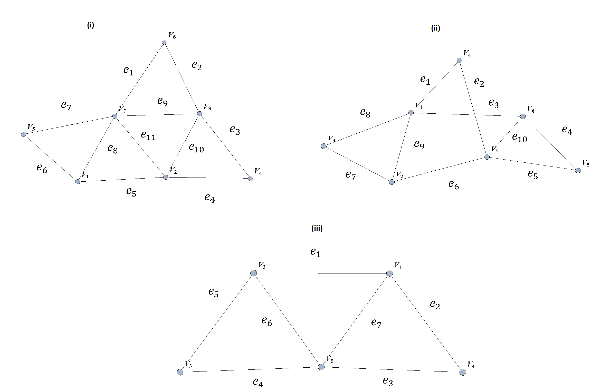
Use the Euler Theorem to explain why the following graphs do not have Eulerian circuits but do have Eulerian paths. Give an Eulerian path for each graph.
Use the Dirac Theorem to explain why the following graphs are Hamiltonian (have Hamiltonian circuits). Provide a Hamiltonian circuit for each graph.
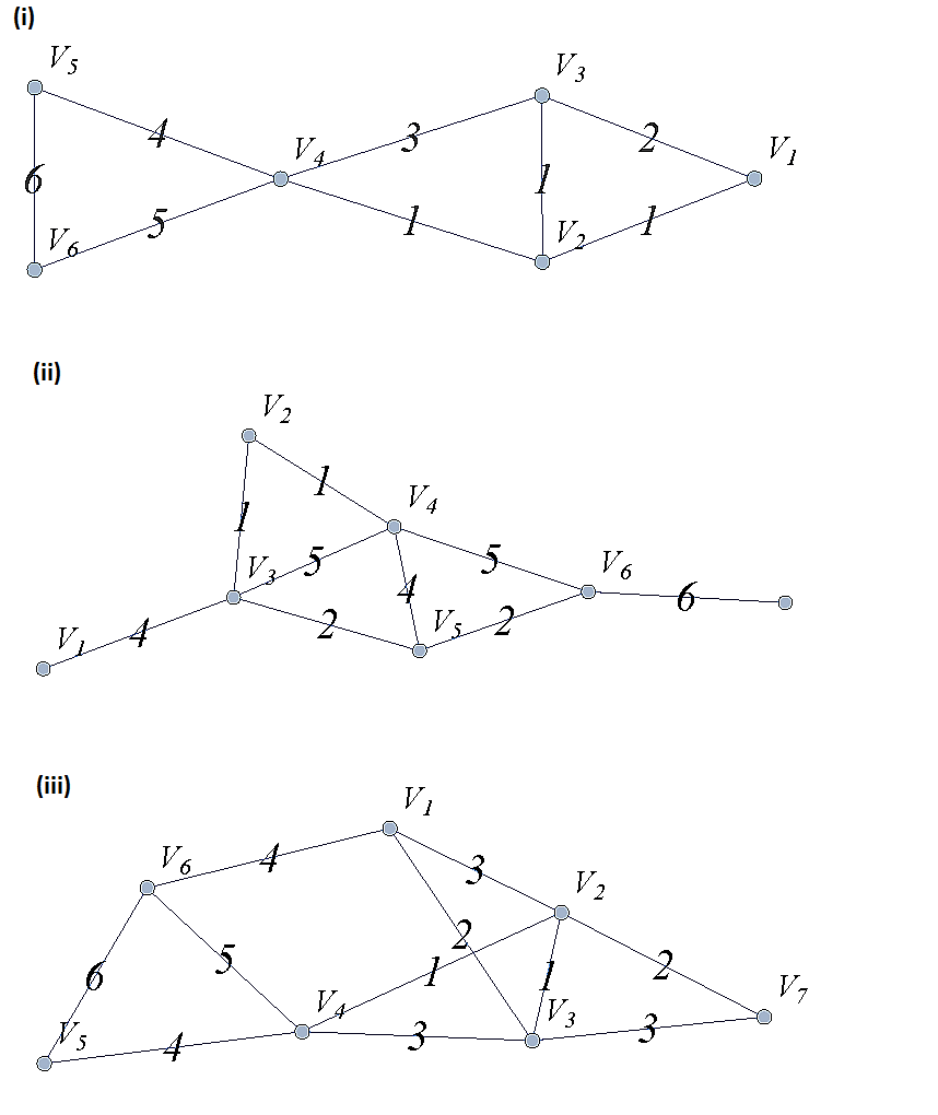
A spanning tree on a graph \(G\) with \(n\) vertices is a subgraph of \(G\) with \(n-1\) edges that form a tree. For a weighted graph, the minimum spanning tree is a spanning tree with minimum total edge weights. Kruskal’s algorithm is a procedure that finds the minimum spanning tree for a weighted graph. It sorts the edges in nondecreasing order by weight and then builds the minimum spanning tree, beginning just with the vertices (technically called a forest), and then successively adding edges of nondecreasing weights that do not form cycles. Formally the Kruskal algorithm is,

(1) Choose an edge with minimum weight and add it to the tree provided it does not create a cycle.

(2) Choose an edge with minimum weight and add it to the tree provided it does not create a cycle.

(3) Repeat step (2) until \(n-1\) edges are added to create a spanning tree of \(n-1\) edges.

Apply Kruskal’s algorithm to the following graphs.