Discrete Math

13.1. Quadratic Function

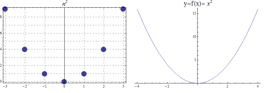
The function $f(x) =x^2$, denotes the association $(a,b) =(x, x^2)$ with $f : \mathbb{R} \rightarrow \mathbb{R}$. We notice that the range is the set of real numbers $[0, \infty)= \mathbb{R}^{+}$. The function is not invertible, since it is not injective. For example, we have both $f(-3) =9$ and $f(3)=9$. With $f : \mathbb{Z} \rightarrow \mathbb{Z}$ notice that the range is now $\mathbb{N}$

\begin{array}{lccccccccccc} & x & -5 & -4 & -3 & -2 & -1 & 0 & 1 & 2 & 3 & 4 & 5 \\ & x^2 & 25 & 16 & 9 & 4 & 1 & 0 & 1 & 4 & 9 & 16 & 25 \end{array}

The graph of $x^2$

13.2. The Cubic function

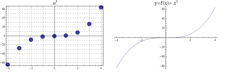
The function $f(x) =x^3$, denotes the association $(a,b) =(x, x^3)$ with $f : \mathbb{R} \rightarrow \mathbb{R}$. Also, we notice that the range is the set of all real numbers $(- \infty , \infty)=\mathbb{R}$. The function is bijective and so invertible. With $f : \mathbb{Z} \rightarrow \mathbb{Z}$, notice that the range, in addition to domain, is also $\mathbb{Z}$

\begin{array}{llcccccccccl} & x & -5 & -4 & -3 & -2 & -1 & 0 & 1 & 2 & 3 & 4 & 5 \\ & x^3 & -125 & -64 & -27 & -8 & -1 & 0 & 1 & 8 & 27 & 64 & 125 \end{array}

The graph of $x^3$

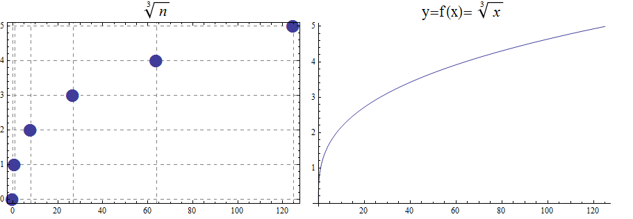
13.3. The Square Root and Cube Root Functions

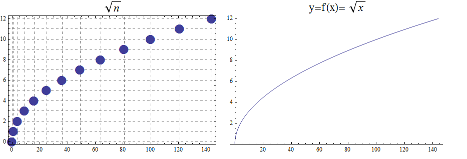
For the purposes of completeness and for comparing how fast functions $f(x)$ grow for large x, we present the inverse of the functions $f(x)= x^2$ and $f(x)= x^3$, when $f(x):\mathbb{R}+→\mathbb{R}+$. Respectively, the functions$ f(x)=\sqrt{x}$ and $f(x)= $ \$root(3)(x)\$.

\begin{array}{lcccccccccclll} & x & 0 & 1 & 4 & 9 & 16 & 25 & 36 & 49 & 64 & 81 & 100 & 121 & 144 \\ & \sqrt{x} & 0 & 1 & 2 & 3 & 4 & 5 & 6 & 7 & 8 & 9 & 10 & 11 & 12 \end{array}

The graph of $√x$

\begin{array}{lcccccl} & x & 0 & 1 & 8 & 27 & 64 & 125 \\ & \sqrt[3]{x} & 0 & 1 & 2 & 3 & 4 & 5 \end{array}

The graph of \$root(3)(x)\$

13.4. Exponential and Logarithmic Functions

We begin by summarizing important properties of exponentials.

Properties of Exponentials

For $a>0, a ≠ 1$, $a^m.\ a^n=a^{m+n}$. For example, $3^4\cdot 3^5=3^{4+5}=3^9$.
$\frac{a^m}{a^n}=a^{m-n}$. For example, $\frac{3^5}{3^2}=3^{5-2}=3^3 $.
$\left(a^m\right)^n=a^{m.n\ }$. For example, $\left(3^4\right)^3=3^{4\cdot 3}=3^{12}$.
$\left(a.b\right)^m=a^mb^m$. For example, $\left(3x\right)^4=3^4.x^4$
$a^0=1$
$a^{-1}=\frac{1}{a}$ For example, $3^{-1}=\frac{1}{3}$.
$ a^\frac{1}{n}=root(n)(a)$.

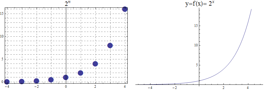
13.4.1. Exponential Functions

Exponential functions are of the form $f\left(x\right)=b^x$, where $b$ is the base and the variable $x$ is in the exponent. The base $b>0$ and $b ≠ 1$. Properties of exponential functions come from properties of exponents. When the base $b$ is greater than 1 the exponential function is increasing exponentially, as in the case $f(x) = 2^x$.

\begin{array}{llcccccccccl} & x & -5 & -4 & -3 & -2 & -1 & 0 & 1 & 2 & 3 & 4 & 5 \\ & 2^x & \frac{1}{32} & \frac{1}{16} & \frac{1}{8} & \frac{1}{4} & \frac{1}{2} & 1 & 2 & 4 & 8 & 16 & 32 \end{array}

The graph of $2^x$

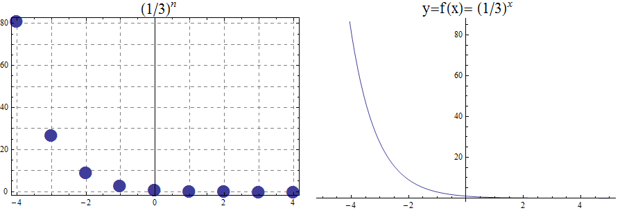
When the base $b$ is less than 1 the exponential function is decreasing exponentially, as in the case $f(x) = \left(\frac{1}{3}\right) ^x$.

\begin{array}{llcccccccccl} & x & -5 & -4 & -3 & -2 & -1 & 0 & 1 & 2 & 3 & 4 & 5 \\ & (\frac{1}{3})^x & 243 & 81 & 27 & 9 & 3 & 1 & \frac{1}{3} & \frac{1}{9} & \frac{1}{27} & \frac{1}{81} & \frac{1}{243} \end{array}

The graph of $\left(\frac{1}{3}\right)^x$

13.4.2. Logarithmic Functions

Logarithmic functions are the inverse functions corresponding to exponential functions and are used to solve exponential equations. For example, $y=2^x$ is solved for $x$ by inverting $x=\log_2{y}$. Properties of logarithms follow from this relationship between exponentials and logarithms and properties of the exponentials.

We summarize three important properties of logarithms.

Properties of Logarithms

The exponential function $f\left(x\right)=y=b^x$, written in exponential form is $\log_b{f\left(x\right)=\log_b{y=x}}$. Its inverse is the logarithmic function $x=b^y$, which is denoted $y=\log_b{x}$.
The power rule for logarithms states that $\log_b m^x=x\cdot \log_b m$.
Comparing the solutions of $2^x$, $x=\log_2{5}\text{,}$ and $x=\frac{\log_{10}{5}}{\log_{10}{2}}$, gives $\log_2{5}=\frac{\log_{10}{5}}{\log_{10}{2}}$, which, essentially, is the change of base formula $\log_b{A}=\frac{\log_a{A}}{\log_a{b}}$.

All other properties of logarithmic functions come from properties relating the logarithm as the inverse of the exponential and the equivalence of the logarithm $a =\log_b m$ with $b^a=m$.

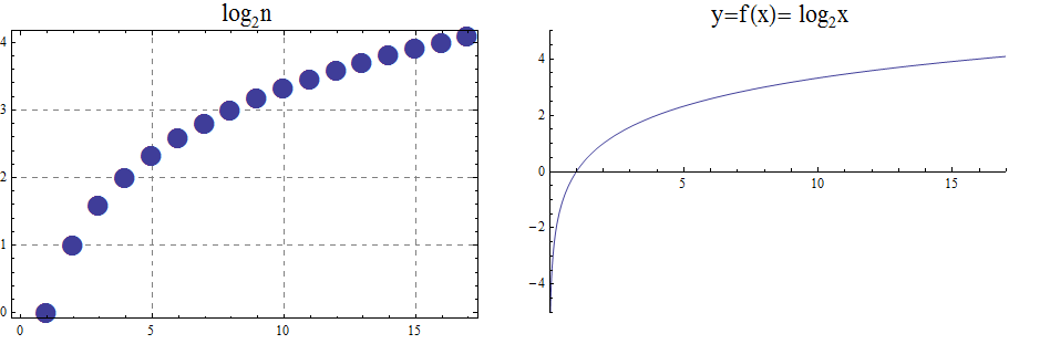
When the base $b$ is greater than 1, the logarithm function is increasing, as in the case $f(x) = \log_2 x$.

\begin{array}{llllllcccccc} & x & \frac{1}{32} & \frac{1}{16} & \frac{1}{8} & \frac{1}{4} & \frac{1}{2} & 1 & 2 & 4 & 8 & 16 & 32 \\ & log_2 x & -5 & -4 & -3 & -2 & -1 & 0 & 1 & 2 & 3 & 4 & 5 \end{array}

The graph of $\log_2 x$

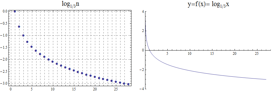
When the base $b$ is less than 1, the logarithm function is decreasing exponentially, as in the case $f(x) = \log_{\frac{1}{3}} \ x$.

\begin{array}{llllllcccccl} & x & \frac{1}{243} & \frac{1}{81} & \frac{1}{27} & \frac{1}{9} & \frac{1}{3} & 1 & 3 & 9 & 27 & 81 & 243 \\ & \log_{\frac{1}{3}} x & 5 & 4 & 3 & 2 & 1 & 0 & -1 & -2 & -3 & -4 & -5 \end{array}

The graph of $\log_{\frac{1}{3}} \ x$